TPP Tutorial v1
From SPCTools
Trans Proteomic Pipeline (TPP) Tutorial
TPP V3.2.1, 2007. Note: Screenshots may vary from the TPP build you are using because the application is in development.
This document was originally assembled by Bryan Prazen of Insilicos.
Contents |
Introduction
This tutorial will cover the application of the Trans Proteomic Pipeline (TPP) for protein identification and quantitation to LC-tandem MS data. The data used in this tutorial has previously been searched with SEQUEST (Thermo Finnigan). Although this tutorial should be helpful to anyone interested in statistical identification and quantitative analysis of proteins with mass spectrometry, this tutorial was designed for the scientist who is currently running SEQUEST searches on their tandem mass spectrometry data and would like to process their data a step further. This tutorial shows an example of how to run the TPP tools so that searched data can be statistically evaluated, quantified and organized using TPP. This tutorial focuses on the application of TPP and only briefly touches on the bioinformatics behind the tools which are included in TPP.
About Trans-Proteomic Pipeline
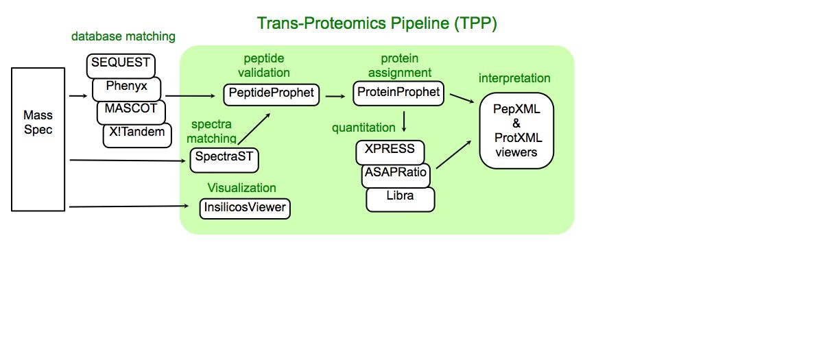
Trans-Proteomic Pipeline (TPP) is a data analysis pipeline for the analysis of LC/MS/MS proteomics data. TPP includes modules for validation of database search results, quantitation of isotopically labeled samples, and validation of protein identifications, as well as tools for viewing raw LC/MS data, peptide identification results, and protein identification results. The XML backbone of this pipeline enables a uniform analysis for LC/MS/MS data generated by a wide variety of mass spectrometer types, and assigned peptides using a wide variety of database search engines.
Systems Requirements
This tutorial does not require a search engine. Searched data is provided. A computer running Windows, XP or 2000 is required. Currently builds of TPP are distributed for Linux and native Windows. This tutorial focuses on TPP run in the Windows operating system. A web browser such as Firefox or Internet Explorer is required. Including the TPP software, the tutorial requires about 900MB of hard drive space. TPP itself requires approximately 190MB of disk space. The remaining space is necessary to store and manipulate the data. For TPP analysis of your data it is important to remember that TPP requires that mass spectrometer data be saved in mzXML or mzDATA formats. mzXML and mzDATA are instrument independent data formats used by data analysis software like TPP and data repositories. mzXML was developed by the Institute for Systems Biology and mzData, developed by the HUPO PSI standards group. Unfortunately, storing data in both the mass spectrometer manufacture specific format and one instrument independent data format will require more than twice as much storage space for data.
About this Tutorial
This guide uses the following typographical conventions: Bold is used to indicate commands or steps that the user must complete. Small Itallics is use for notes that contain information that is not required to complete this tutorial.
Who Should Use this Tutorial?
This tutorial is written for anyone who has a general interest in learning about one method to identify and quantify peptides and proteins using mass spectrometry. We have attempted to write this tutorial so that the user does not need an extraordinary knowledge of proteomics, biology, chemistry, mass spectrometry, or software engineering. Also, this tutorial does not require any software or data that is not easily available on the web and it does not require any previous experience with the analysis of mass spectrometric data. This tutorial should also be of use to those who are very familiar with proteomics data analysis but do not have a great deal of experience with TPP.
Getting Started
Downloading and Installing TPP
Information on installing and downloading the Windows distribution of TPP can be found at: sourceforge
Setting up an account
The TPP GUI comes with one user account. This account has ‘guest’ as both the user name and password. Below are instructions for making another account from a Cygwin shell. The Cygwin Bash Shell can be found under Cygwin in the Windows start menu.
Open the DOS shell by selecting Run under the Start menue and typing cmd. In the shell type:
cd c:\Inetpub\tpp-bin\users\
mkdir tutorial
cd tutorial
crypt isbTPPspc TPP > .password
and
chmod -R 777 C:\Inetpub\tpp-bin\users\tutorial
You have just created the password ‘TPP’ for the user ‘tutorial.’
In order to add a different username, create a tpp-bin/users/NEWUSER/ directory and run crypt isbTPPspc NEWPASSWORD > .password from this directory. In these examples "isbTPPspc" is the crypt key. This can be changed.
Tutorial Data
Getting the Tutorial Data
This tutorial uses a data set containing proteins that co-purified with lipid raft plasma membrane domains isolated from control and stimulated Jurkat human T cells. The analysis of similar data can be found in:
“The Application of New Software Tools to Quantitative Protein Profiling Via Isotope-coded Affinity Tag (ICAT) and Tandem Mass Spectrometry: II. Evaluation of Tandem Mass Spectrometry Methodologies for Large-Scale Protein Analysis, and the Application of Statistical Tools for Data Analysis and Interpretation” Priska D. von Haller, Eugene Yi, Samuel Donohoe, Kelly Vaughn, Andrew Keller, Alexey I. Nesvizhskii, Jimmy Eng, Xiao-jun Li, David R. Goodlett, Ruedi Aebersold, and Julian D. Watts, Mol Cell Proteomics 2003 2: 428-442."
The data used in this tutorial is not the same data that is described in the publication but the same scientists collected it using the same sample preparation and mass spectrometry procedures. Analysis was done on a LCQ Classic. The samples were ICAT labeled (Old-ICAT, light tag = d0 442, heavy tag = d8 450), separated by cation exchange chromatography, purified by avidin cartrages, separated by μLC, and measured with MS/MS. The tandem mass spectra were then analyzed using SEQUEST. This tutorial begins with the analysis of the SEQUEST results. Only a portion of the data from the raft experiment is used in this tutorial in order to save time and hard drive space. This tutorial uses data that has already been searched by SEQUEST so that the user does not need to have a SEQUEST license for the computer that is used for this tutorial.
Download this data at:
www.insilicos.com/spctools/data/tutorial_wiki.exe
Tell your browser to save the file. The download is a self extracting compressed folder. Run the download to extract the data to C:\Inetpub\wwwroot\ISB\data\tutorial.
Unpacking and Storing the TPP Tutorial Data
It is important that all the data that is analyzed with the TPP be stored in specific locations. The TPP can only see data that is located under the C:\Inetpub\wwwroot\ISB\data directory.
For this tutorial and future data analysis all data should be stored in C:\Intetpub\wwwroot\ISB\data\. Each experiment can be stored in an individual folder at this location, such as our tutorial folder.
You should now have a folder named ‘tutorial’ which contains mzXML data for 6 LC runs, folders that contain the .out and .dta files, a sequest.params file and a folder containing a FASTA database.
NOTE: To analyze data from your own experiments you will need to search the data, compress the search results and convert the raw data to mzXML format. These steps are covered in the last section - Beyond this Tutorial. The dbase folder needs to be somwhere that TPP can find it.
Move the dbase folder to C:\Inetpub\wwwroot using windows Explorer.
Many problems with TPP are associated with file permissions and these problems seem to be very machine dependent. We will start by changing the permissions of your data folder. Type the following command in the DOS shell:
chmod -R 777 C:\Inetpub\wwwroot\ISB\data\tutorial
chmod -R 777 C:\Inetpub\wwwroot\dbase
For other permission related problems type the same command with the appropriate directory inserted.
SEQUEST data analysis
Opening the GUI
The TPP pipeline GUI can be opened by clicking on the ‘TPP Web Tools’ shortcut that was created on your desktop during installation or by selecting “TPP Web Tools” under “TPP” in the Windows start menu. Alternatively, you can click on the following link or open your favorite web browser and paste this link into the navigation bar:
http://localhost/tpp-bin/tpp_gui.pl
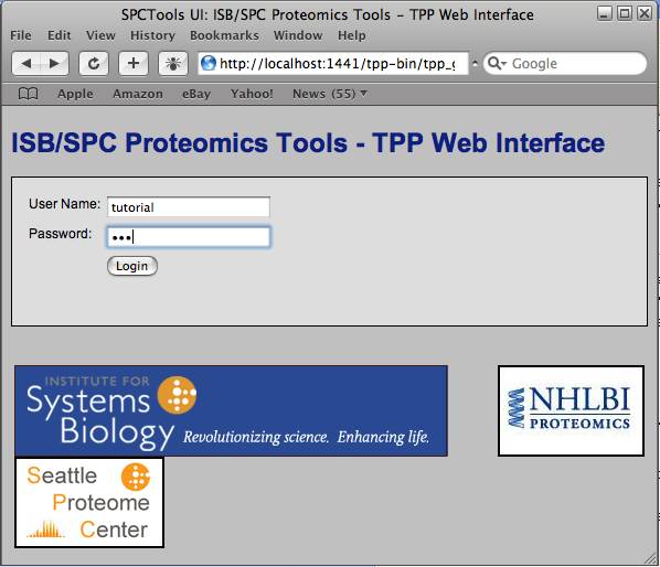
Login as ‘tutorial’ and use ‘TPP’ as the password.
This tutorial is written from the point of view of a researcher viewing data on the computer where the TPP tools are running.
At this point you will be in the “Home” tab of the proteomics pipeline GUI. The Home tab contains information about TPP and the structure of the GUI, along with a pull down menu that lets you choose between SEQUEST, Mascot, Tandem or SpectaST. The default is SEQUEST which is what will start with in this tutorial. Thus, no input is necessary under this tab.
Creating pepXML Files
For this tutorial we begin with data that has already been searched with SEQUEST so that the tutorial is instrument independent and does not require software beyond TPP. The SEQUEST Search results are in the form of .out files. TPP will analysis the search results in pepXML format. The next step will be to convert the .out files to pepXML files.
Click on “Analysis Pipeline”. This will display six tabs which activate different parts of the pipeline. The first tab is Home, which contains information about the TPP. The second tab is used to convert data from different spectrometers into mzXML, and the third tab is used to search the data. We will start with the pepXML tab. Your next step is to convert the search results from .out to the pepXML format. pepXML is a file format for storing the results of database search at the peptide level. A great thing about pepXML is that its format is independent of the instrument manufacture and database matching software. pepXML converters are currently available for SEQUEST, Mascot, COMET and X!Tandem results. Also, the Mascot software contains a pepXML exporter.
NOTE: In the near future look for the mzIdent file format that will be a Human Proteome Organisation (HUPO) standard based on pepXML.
Select the ‘pepXML’ tab in the GUI interface.
Select the ‘Add Files’ button.
Using the directory selector on the right side, navigate to the tutorial directory.
Check the select box to the left of each of the 6 .out folders
Press the ‘Select’ button.
In the updated window,
Press ‘Add Files’ under the ‘Specify Sequest Parameters File’ section.
Check the sequest.params file and press ‘Select’.
There is no need to select any of the options and the enzyme should already be set as trypsin.
Press ‘Convert to PepXML’.
This command will take a moment to run. Select the Show Command Status link. You will need to update the page by clicking the text “UPDATE THIS PAGE”. When the command is completed The Command Status area will have the message "Your commands have finished executing."
Select the "View results of previous commands" link in the Command Status section.
At this point you have successfully converted your search results to the pepXML format and you are ready to evaluate your data with the tools that are included in TPP.
NOTE: When analyzing your own data, the working directory must contain the spectra (.mzXML, mzDATA or .mzML) and the SEQUEST results in .tgz or subdirectorys for Sequest2XML to work.
PepXML files contain information about peptides derived from tandem MS data. PepXML files are iteratively modified by various programs as processing progresses. A basic PepXML file, like the six that you just created contain only search-engine results. After further processing the pepXML file will also contain the results from these processes.
PepXML Viewer
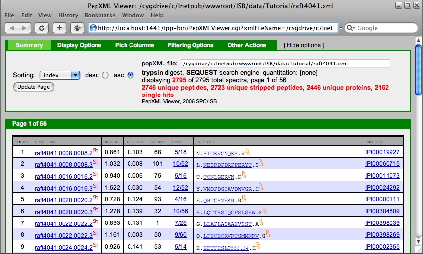
The pepXML viewer is another application that runs through your web browser. The pepXML viewer allows you to filter, sort and view your search results. From the Output Files tab that appears after the data conversion has completed and you have updated the page, Click the ‘PepXML’ link next to the raft4041.xml.
NOTE: This window can also be accessed by typing the following link in your web browser http://localhost:1441/ISB/Tutorial/raft4041.xml.
A new window containing a pepXML viewer will open. From here you can generate a Pep3D image of the LC/MS data, view the complete SEQUEST output for any spectrum, look at the spectra with the matching ions highlighted, see the peptide in relation to the protein it is part of, BLAST the protein, filter the results and sort the results.
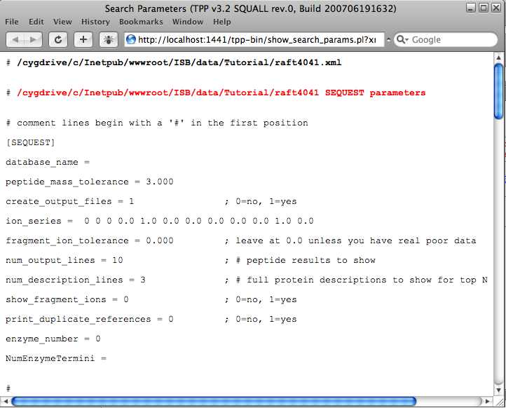
Under the Other Actions tab there is an Additional Analysis Info button. Select these and the SEQUEST link to view the SEQUEST parameters. This will give you an idea how the the search was done.
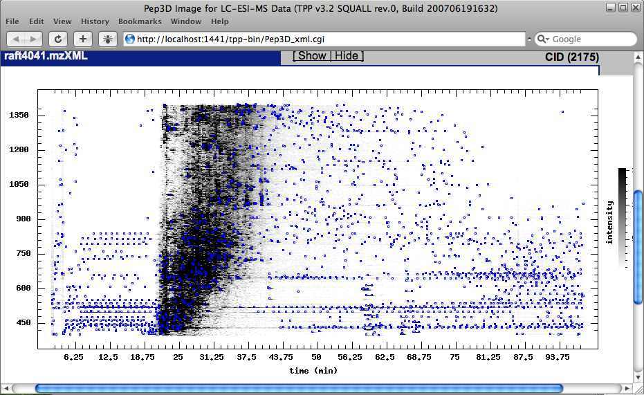
Another button under the Other Actions tab is the Generate Pep3D image button. Click on the ‘Generate Pep3D’ button. When the Pep3D parameters page appears, leave the default parameters and select the 'Generate Pep3D image' button. Pep3D images can be very useful in assessing the quality of the LC-MS/MS data. The Pep3D map has mass channels on one axis and chromatographic time on the other. Blue dots represent locations where tandem MS were collected. The Pep3D image has interactive control of the display.
Returning to the pepXML viewer, the “index” column is a unique search result id.
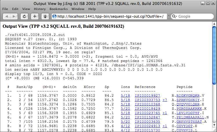
The “spectrum” column contains the name of the .out file resulting from the SEQUEST search and links to comprehensive search results, including runner up peptides. Click on the “spectrum” entry for the first peptide assignment. This does not give you an actual mass spectrum, but instead a new window containing the SEQUEST results for that peptide assignment. This can be useful for curating the data. For instance the fact that none of the close matches have tryptic termini in this example is further assurance that the assignment is correct.
The ST symbol next to the spectrum link links to an automated spectrum posting for Spectra Search Tool (SpectraST) at PeptideAtlas. PeptideAtlas is a data repository and SpectraST is an alternative to search engines like SEQUEST which matches data to a library of spectra. Spectral library searching, unlike sequence database searches, involve finding the best match of an acquired MS/MS spectrum to a library of pre-searched spectra for which the sequences have been determined. This approach can be hundreds of times faster than traditional searching, with comparable or better accuracy. Clicking on the ST symbol allows you to donate your spectrum to the spectrum library at PeptideAtlas.
The “xcorr”, “deltacn” and “sprank” columns on the pepXML viewer are results from the SEQUEST search. These columns are specific to each search engine. XCorr is the cross-correlation of the experimental and theoretical spectra. deltaCn is the normalized difference of XCorr values between the best sequence and the next best sequence. Thus, deltaCn is a measure of the uniqueness of the match. DeltaCn values that are marked with a star indicated that the second best matching peptide to that spectrum, has >70% sequence similarity with the top match. This can be referred to as a homologues peptides. For the stared values, deltaCn is computed not as a difference between the top score and the second best score, but as a difference between the top score and the score of the first non-homologues peptides. If deltaCn > 0.2 it is colored in pink, for some historic reason. Sprank is the rank of the match in SEQUEST’s preliminary score (sp). Sp is the sum of the peak intensities that match the library peptide and accounts for continuity of an ion series and the length of the peptide.
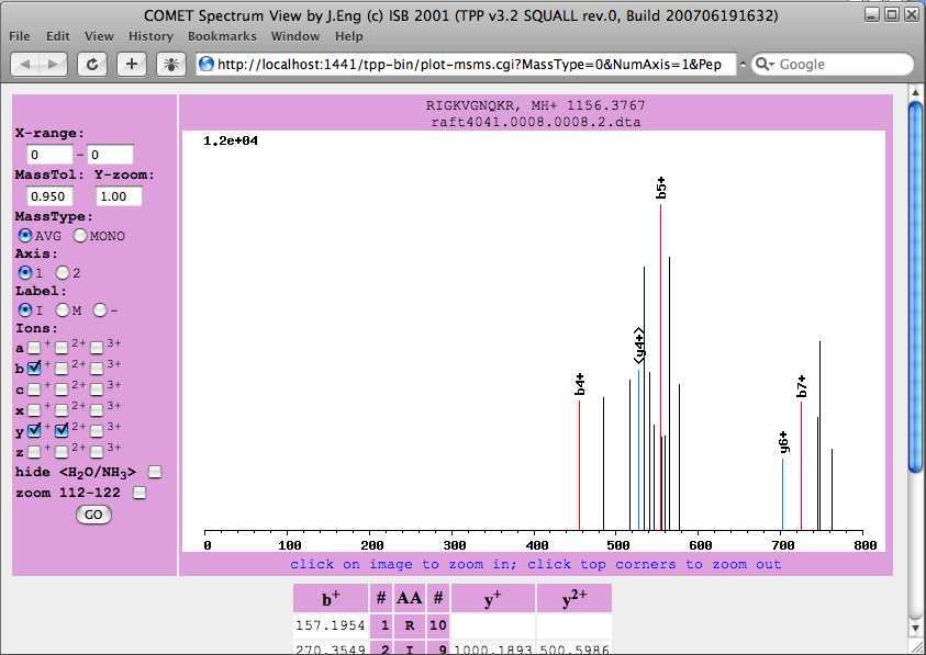
The “ions” column contains the fraction of peptide theoretical fragment ions present in spectrum and links to MS/MS spectrum with assigned fragment ions. Select the “ions” for the first peptide assignment. This displays a mass spectrum for the first peptide assignment. The COMET Spectrum Viewer will be opened. This window is interactive, allowing you to zoom and select the type of ions to highlight. Again this is another tool to evaluate the peptide assignment. Below the spectrum is the amino acid sequence of the matched peptide paired with the weights of the fragments resulting from a break of the peptide at the amino acid. The mass signals found in the spectrum are highlighted. If the matched peptide contains modifications specified in your search you will see the modifications below the list of amino acids in the matched peptide.
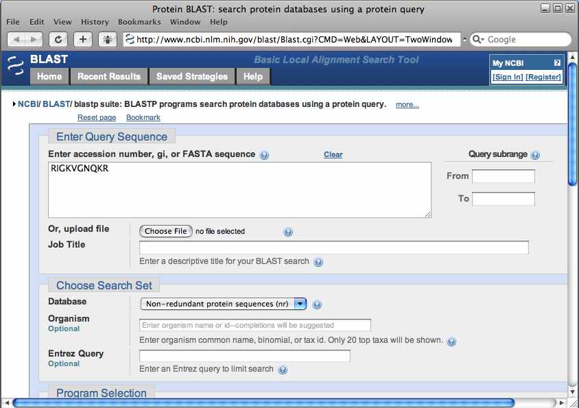
Returning to the PepXML viewer, select a value in the “peptide” column for the first match to open a window for doing a BLAST search of the peptide.
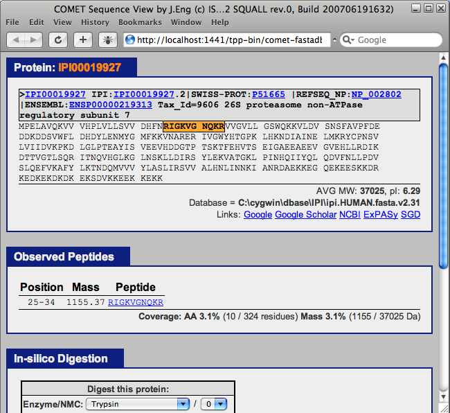
The “protein” column in the PepXML viewer contains the International Protein Index and links to the FASTA database. Select the first value in the “protein” column to open a window containing the COMET sequence viewer. This tool shows the location of the assigned peptide in the protein that contains it. Additional proteins containing the assigned peptide are also displayed.
The "Pick Columns" tab in the PepXML viewer allows you to change the information the is displayed about each match. For instance you could add the "num_tol_term" column to display the number of tryptic termini in the matched peptide.
Peptide Level Analysis
Now that you have successfully converted your data to the pepXML format, return to the TPP GUI and select the ‘Analyze Peptides’ from under the 'Analysis Pipeline (Sequest)' link.
PeptideProphet
Press the Add Files button.
Check the select box to the left of each of the 6 pepXML files, and press the ‘Select’ button.
In the ‘Output File and Filter Options’, change the ‘Write output to file’ name to raftTPP.pep.xml.
The name interact.xml is too generic. With interact.xml as the name you risk overwriting results when doing multiple analyses. Leave the probability filter at 0.05. This removes some of the very poor search results and makes the data set size more manageable.
Check ‘Run PeptideProphet’ and ‘Use ICAT information’ under the ‘PeptideProphet Options’.
PeptideProphet is a statistical approach for the validation of peptide identifications made by MS/MS searches. By employing database search scores, number of tryptic termini, number of missed cleavages, and other information, PeptideProphet learns to distinguish correctly from incorrectly assigned peptides in the data set and computes for each peptide assignment to an MS/MS spectrum a probability of being correct. It has been shown that using the probabilities computed from the model, one can achieve much higher sensitivity for any given error rate compared to the results of using conventional filtering criteria. The method enables high-throughput analysis of proteomics data by eliminating the need to manually validate database search results. In addition, PeptideProphet results can facilitate the benchmarking of various experimental procedures and serve as a common standard by which the results of different experimental groups can be compared (1).
XPRESS
Under ‘XPRESS Options’:
check the ‘RUN XPRESS’ select ‘C’ for the first labeled amino acid enter ‘8’ for the first mass difference
The TPP contains two tools for quantification of proteins on ICAT-reagent or SILAC (Stable Isotope Labeling with Amino acids in Cell) labeled samples: XPRESS and ASAPRatio. XPRESS Software:XPRESS is a program that calculates the relative abundance of proteins, by reconstructing the light and heavy elution profiles of the precursor ions and determining the elution areas of each peak. To construct the profiles it starts at the MS/MS scan number where the peptide was identified and finds the local minimum to the left and right of this point. XPRESS allows the specification of which residues are labeled (such as cysteines for ICAT) and the mass difference of the two isotope labels (such as 8 Da for old ICAT data) (2). XPRESS was the first of the two quantification methods, but some users find the simplicity of the XPRESS algorithm leads to better results.
NOTE: Because it is difficult for the program to determine the elution profiles I would not recommend the elution time difference option unless there is an unusually big difference in the elution time between the light and heavy peptides.
ASAPRatio
Under ‘ASAPRatio Options’, check ‘RUN ASAPRatio’.
Similar to XPRESS, Automated Statistical Analysis on Protein Ratio (ASAPRatio) calculates the relative abundances of proteins and the corresponding confidence intervals from ICAT or SILCA type ESI-LC/MS data. ASAPRatio Software:ASAPRatio first uses a Savitzky-Golay smoothing filter to reconstruct LC spectra of a peptide and its partner in a single charge state, subtracts background noise from each spectrum, and calculates light:heavy ratio of the peptide in that charge state. The ratios of the same peptide in different charge states are averaged and weighted by the corresponding spectrum intensity to obtain the peptide light:heavy ratio and its error. Subsequently, all unique peptides identified for a given protein are collected, their ratios and errors calculated, outliers are checked for using Dixon's tests, and the relative abundance and confidence interval for the protein are calculated by applying statistics for weighed samples. A byproduct of the software is to identify outlier peptides which may be misidentified or, more interestingly, post-translationally modified. ASAPRatio goes beyond XPRESS in that does background subtraction, error analysis, and provides a criterion for protein profiling (3).
Libra
A third quantitation tool within the TPP is named Libra. Libra performs quantitation on MS/MS spectra that have multi-reagent labeled peptides such as iTRAQ labeled samples. Libra will not be covered in this tutorial because the tutorial data was only labeled with ICAT reagents.
Run Analysis
And finally under ‘Run Analysis’, click the ‘Run Xinteract’ button
Running all of these data processing steps will take about 7 minutes on an average computer. The ASAPRato program is an especially long process. During this time you will have a message that your commands are running. The browser might not refresh when the commands are finished.
Press refresh on the browser to check the status of the analysis.
Select the Show button for the Comand Status.
To speed the process you might try increasing the probability filter (currently set at 0.5).
If you were running TPP from the command line this same operation would have been done using the following commands:
xinteract -NraftTPP.xml -Oi -X-m1.0-nC,8 -A-1C-mC8 *.xml
Bold text==Evaluating the Results of Peptide Level Analysis== Click the "Show" next to the Command Status and wait for the analysis to run. When the process is finished, Press ‘Click here to view log file and output files’ and then press ‘c:\Inetpub\wwwroot\ISB\tutorial\raftTPP.shtml [ View ]’
At this point the number of search results will be reduced to the more manageable number of 542 by the elimination of those with very low PeptideProphet probabilities.
The pepXML viewer contains the controls for filtering and sorting the data. Comparing to the browser window before analysis you will notice that three columns have been added: PROBIBILITY, XPRESS and ASAPRatio.
Click the "other Actions" tab and the “Help” button in the pepXML Viewer. This will open a new widow that contains a detailed explanation of the PepXML Viewer.
PeptideProphet Results
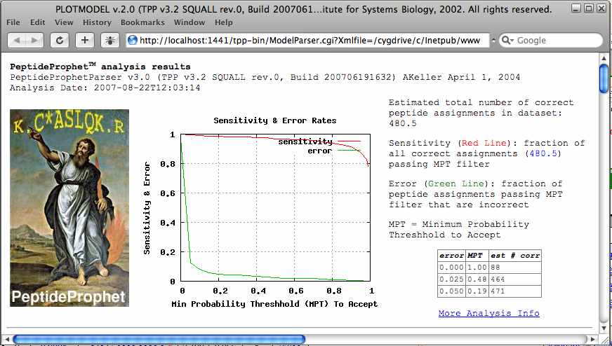
The “PROBABILITY” column is the probability that search result is correct as determined by PeptideProphet. Click on the “PROBABILITY” entry for the first peptide assignment. A new window will open the PLOTMODEL viewer. PLOTMODEL will show the PeptideProphet analysis results.
The top graph in this window shows how sensitivity and selectivity are affected by the probability threshold that the researcher uses to distinguish correct and incorrect identifications. The table to the right of this graph gives three examples of the relationship between the number of peptides assigned and the level of error.
The lower graphs show how well the data (black line) follows the PeptideProphet modeling of the combined XCorr, deltaCn and Sprank (violet and blue lines). Along with the Sequest results (XCorr, deltaCn and Sprank) PeptideProphet uses attributes like the number of tryptic termini, the mass difference of the parent ion, and the number of missed cleavages to determine the probability for a given peptide assignment. With the exception of the red line that indicates the location of this result the graphs are the same for each peptide assignment in the list. This is because the graphs reflect the PeptideProphet model and PeptideProphet uses all the search results to develop the model.
Many people ask questions about how to read PeptideProphet and ProteinProphet probabilities. There is no recommended probability cutoff because this depends on the sensitivity and error rate that you are willing to accept in your result. The prob window will take you to a plot of the expected sensitivity and error rates for various min probability thresholds that are calculated from the corresponding dataset given the model learned by PeptideProphet.
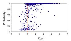
In the pepXML viewer, return to the Summary tab and select Sorting by xcorr, change the radio button on descending (desc) and press ‘Update Page’. If you look through the results you will see that prob values do correlate with xcorr values but they are not perfectly correlated. For instance if you go to page 10 and scroll down to XCorr 1.998 you will see an example of a search with a XCorr below the common threshold of 2.0 but with a probability of 0.88. Yet just a few XCorr down from this one you will see a peptide identification with an XCorr of 1.976 but a probability of only 0.08. Then on the same page if you look up to xcorr 2.110 you will see a petide that only has a probability of 0.06. This poor correlation is a perfect example of the importance of PeptideProphet.
A graph of the relationship between XCorr and probability for the tutorial data is shown below. Notice that the peptide identifications that have XCorr less than 2.0 have a huge range of probabilities.
Next, select Sort by index, ascending and return to the first page. Notice that some of the amino acids in the “peptide” column are marked with a “C553.34” This indicates a heavy labeled cysteine (103(cysteine)+442(ICAT)+8(deuterium) = 553 Da). In the next steps of this tutorial we will see that cysteine containing peptides can be quantified by comparing the chromatographic profiles of the heavy ICAT and light ICAT ions. Note that quantitation can be done on cysteine containing peptides if the light, heavy, or both light and heavy peptides are identified.
Note: For future data sets, if PeptideProphet is unable to find an accurate set of distributions to model a set of identifications in a given charge state, it will display a negative number representing the charge state of the identification. The negative number does not indicate that the match is correct, only that the PeptideProphet could not model the data. This might indicate that there were not enough matches for the charge state in your experiment.
XPRESS Results
As you can see a column containing XPRESS values was added to the pepXML viewer after the analysis was run.
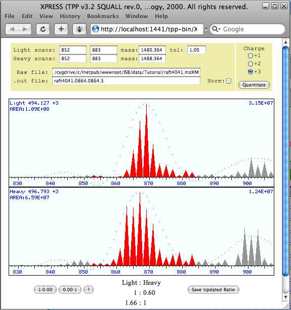
When you have the data sorted by index you will notice that the first peptide match does not have XPRESS ratio. This is because the first peptide does not contain any cysteine amino acids. Click on the first value in the “XPRESS” column. This brings up a window with the chromatographic profiles for the light and heavy ions used for XPRESS quantitation.
From this window you can change the chromatographic elution range and mass that is integrated for quantitation of this peptide. Notice that the same peptides are identified in the 2nd and 3rd spectra when the data is sorted by index, yet one XPRESS ratio is 1:0.61 and the other is 1:0.80. Two values are listed because this peptide was identified from a +2 ion and a +3 ion. Obviously, both ratios cannot be correct. Sort the data by Protein. If you review this data you will see that some proteins have conflicting ratios. As we will see in the next sections the ASAPRatio tool address the issue of variation in ratios for a single peptide and ProteinProphet addresses inconsistency within proteins. The level of agreement between XPRESS ratios can be used to evaluate the precision and accuracy of the quantitation.
ASAPRatio Results
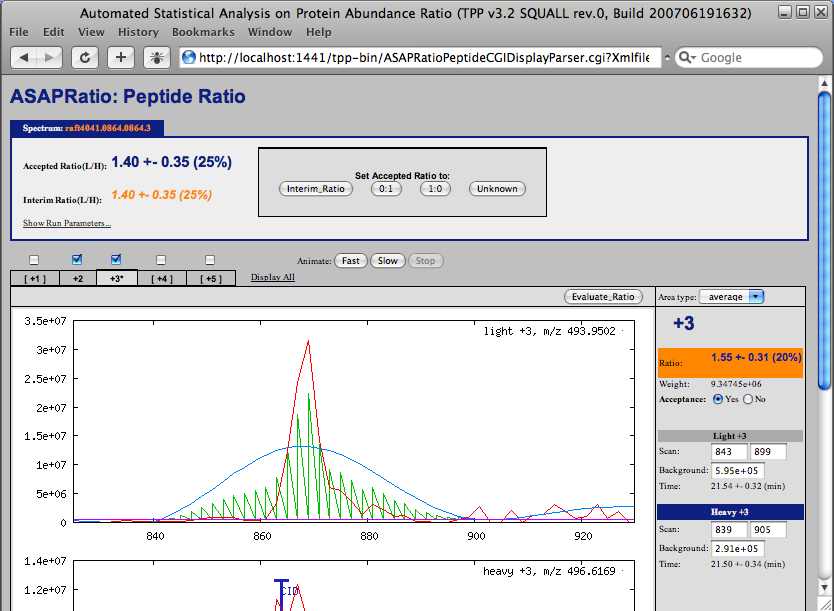
The “asapratio” column contains quantitation results with a link to the ASAPRatio ion trace. The number listed in the “asapratio” column is the light to heavy ratio. Unfortunately this is the reciprocal of the ratio usually listed in the “XPRESS” column. The GUI does have an option to invert the XPRESS or ASAPRatio ratios. You might want to select this option the next time you analyze data.
Click on the first value in the “asapratio” column. Like the “XPRESS” column, this brings up a window with the chromatographic profiles for the light and heavy ions used for quantitation. Also like XPRESS, you can change the chromatographic elution range and mass that is integrated for quantitation of this peptide from this widow. If you scroll through the ASAPRatio results in the pepXML viewer while the data is sorted by Protein you will notice that discrepancies in quantitative ratios for a given peptide are gone, yet discrepancies still remain on the protein level.
Reviewing Processed Data
The GUI is an easy to use tool for running the TPP programs and viewing your results during the process, but what do you do when days after the analysis you realize that you want to go back to that data and sort it a different way, set a different cutoff, or review the ASAPRatio’s chromatographic profile for that surprising result? When we opened the pepXML viewer the GUI displayed the name of the file that was being opened: c:\Inetpub\wwwroot\ISB\data\tutorial\raftTPP.xml. Do not access this file through Windows or paste this file into your browser.
To access this tutorial’s pepXML file through the pepXML viewer:
Open a new window in your browser
Type or paste the following location into the address bar: http://localhost:1441/ISB/data/tutorial/raftTPP.xml
In order to view the data in the pepXML viewer the pepXML viewer must be run through your web server. Thus, the address bar of your browser should never have an address that starts with “C:” or “file:”. Your browser should always have an address that starts with a “http:”. When you are viewing the data from the computer that contains the TPP, http://localhost:1441 leads to the C:\Inetpub\wwwroot\ directory.
You should be aware that as you filter and sort the data in the pepXML viewer, the results of the TPP analysis are being written over. You can always restore the entire original dataset by clicking on the ‘Restore Original’ button under the Other Actions tab, but intermediate processing will be lost.
Protein Analysis
In the TPP GUI, select the ‘Analyze Proteins’ tab.
Then press the ‘Add Files’ button and select the raftTPP.xml file.
Note that for protein analysis you want to select the data the already contains the peptide analysis information. raftTPP.xml contains the peptide analysis results for the analysis of the 6 .xml files combined.
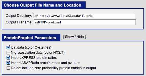
Change the ‘Output file name’ to raftTPP-prot.xml.
Check the ‘ICAT data’ box.
Check the ‘Import XPRESS protein ratios’ box.
Check the ‘Import ASAPRatio protein ratios and pvalues’ box.
Under ‘Run Protein Analysis!’, click the ‘Run ProteinProphet’ button.
ProteinProphet takes the peptides and search results and statistically validates the identifications at the protein level. Different peptide identifications corresponding to the same protein are combined together to estimate the probability that their corresponding protein is present in the sample. This protein grouping information is then employed to adjust the individual peptide probabilities, thus making the approach more discriminative. ProteinProphet also addresses degeneracy, which occurs when one peptide corresponds to several different proteins (4).
After the program completes you should see a message that your commands have finished executing. You may need to refresh the browser to get this message. One way to monitor the progress of any of the TPP tools is to use the Windows task manager’s CPU usage display. The TPP tools will utilize nearly 100% of the available CPU while analyzing the data.
NOTE: To open the Windows Task Manager press Ctrl+Alt+Delete, then select the ‘Performance’ tab.
Click the Show link in the Command Status area.
Press ‘Click here to view log file and output files’ and then press ‘View output files (raftTPP-prot.xml)’.
Notice that this time you are looking at a similar but different viewer. This is the protXML viewer. A different viewer is used because the data is stored in a different XML format after it is combined according to proteins.
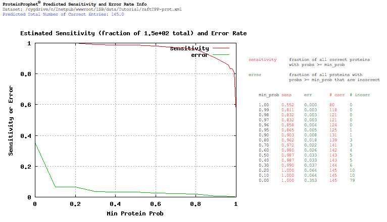
At this point we have focused the data down to the identification and quantitation of 224 proteins. Sort the data by probability. If you scroll down through the proteins you will see that only 155 proteins have a probability above zero and only 131 have a probability above 0.90. Click the ‘Sensitivity/Error Info’ button which is located to the right of the ‘Filter/Sort/Discard checked entries’ button to view a breakdown of the protein identification probabilities from the ProteinProphet analysis. The functions are not very smooth for this data. This is because there are a relatively small number of proteins. Remember we are only analyzing 6 of the 24 separations in from the raft experiment in this tutorial. Also remember that the TPP identification tools build models based on the peptide searches from a given experiment, and a large number of quality searches in a single experiment leads to better models.
If you scroll through the proteins, you will see many proteins with a probability of zero. Most of the cases with a probability of zero contain peptides that are contained in multiple proteins in the database. The weight column for each peptide in the proteins contains a value between zero and one that apportions peptides between possible proteins. Iterative modeling is used to determine the weight such that the total weight for a peptide in all proteins is one, high probability proteins are weighted more heavily, and the simplest list of proteins is created.
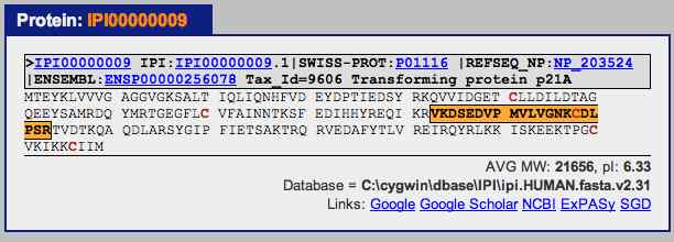
Select the first “International Protein Index (IPI)” for the first protein on the list. This brings up a window showing the protein with its identified peptides highlighted.
Returning to the ProtXML viewer, in red following the IPI is the protein probability. The next information given on the protXML viewer is the percent coverage of the peptides identified in a given protein. This is followed by the XPRESS and ASAPRatio quantitations. Note that at this point a single XPRESS ratio and a single ASAPRatio have been determined for each protein that was identified. The error values listed for the ratios take into account the ratios for different peptides in the protein. You can click on the XPRESS and ASAPRatio values to get further explanation of these results. The “pvalues” column gives the result of a statistical test for the quantitative values.
Exporting Data
At this point in the analysis you are ready for publication. Results shown in the protXML Viewer can easily be exported to an Excel spreadsheet for further sorting, distribution, graphing and publication. Export can also be done at the peptide analysis level using the pepXML Viewer.
From the protXML Viewer, check the ‘Export to Excel’ box and then press the ‘Filter/Sort/Discard’ button to write the filtered dataset out in tab delimited format. The spreadsheet that is written will closely mimic the view of the data in your browser. A link to the written Excel spreadsheet is displayed at the top of the protein list.
Automation
In this tutorial we broke the data analysis into steps so that we could explain the process. When you want to do high throughput uninterrupted data analysis you can use the command line. The following command would take the tutorial data completely through the data analysis pipeline and result in the same answers that were obtained in the tutorial.
xinteract -NraftTPP.xml -p0.05 -Oip -X-m1.0-nC,8 -A-1C-mC8 *.xml
Another way to streamline the process is to do run the peptide level analysis and protein level anlaysis in the same step. You can do this by selecting "run ProteinProphet afterwards" from the PeptideProphet options.
Beyond this Tutorial
Creating mzXML Files
TPP requires the MS/MS data in mzXML format. mzXML is an XML (eXtensible Markup Language) format for mass spectrometric data. Most mass spectrometers do not directly produce mzXML files, but there are several tools available that generate mzXML files from native acquisition files. The second tab on the TPP GUI offers conversion from ThermoFinnigan Xcalibur .RAW files to mzXML.
Currently, there are SPC-developed converters available for ThermoFinnigan Xcalibur, Micromass MassLynx, and SCIEX/ABI Analyst native acquisition files. Most mzXML converters are included in the TPP software package. These include:
- ReAdW: ThermoFinnigan Xcalibur format to mzXML converter (Included in the proteomics pipeline GUI)
- MassWolf: Micromass MassLynx format to mzXML converter
- mzStar: SCIEX/ABI Analyst format to mzXML converter
- mzBruker: Bruker format to mzXML converter (replaced by Bruker's compassXport program, follow link for info.)
References
1
A. Keller, A. I. Nesvizhskii, E. Kolker and R. Aebersold "Empirical Statistical Model To Estimate the Accuracy of Peptide Identifications Made by MS/MS and Database Search" Anal. Chem. 2002, 74, 5383-5392.
2
D. K. Han, J. Eng, H. Zhou and R. Aebersold "Quantitative profiling of differentiation-induced microsomal proteins using isotope-coded affinity tags and mass spectrometry" Nature Biotechnology 2001, 19, 946-951.
3
X.-j. Li, H. Zhang, J. A. Ranish and R. Aebersold "Automated Statistical Analysis of Protein Abundance Ratios from Data Generated by Stable-Isotope Dilution and Tandem Mass Spectrometry" Anal. Chem. 2003, 75, 6648-6657.
4
A. I. Nesvizhskii, A. Keller, E. Kolker and R. Aebersold "A Statistical Model for Identifying Proteins by Tandem Mass Spectrometry" Anal. Chem. 2003, 75, 4646-4658.
